
Home Credit Default Risk
Using Machine Learning to Predict Loan Repayment

Disclaimer: Below is a Machine Learning project done by four IU grad students, myself included. The report below is written by Kaitlin Knecht based on the work we did as a collective.
By Kaitlin Knecht, Thomas Koutsidis, Julia Hoa Nguyen, Mackenzie Ross
Abstract
Home Credit, a financial institution, presents data in Home Credit Default Risk meant for analyzation through machine learning to predict whether or not a client will repay their loan. The purpose of this project is to develop the best machine learning model for this task. Through exploratory data analysis, feature engineering and selection, hyperparameter tuning, and evaluations of a logistic regression model, a support vector machine model, and a neural network, this task was accomplished. It was found that a support vector machine model with a radial basis function kernel and C=1 best predicted the data provided. The results of this model include: training accuracy 92.88%, validation accuracy 91.77%, and test accuracy 89.85%. Additionally, the corresponding test area under the receiver operating characteristic curve scored 0.67. In the Kaggle competition submission, public and private scores of 0.5 were achieved.
Introduction
Home Credit is a financial institution that, among other things, provides their clients with loan services. There are clients that are not given a loan because they do not meet the minimum requirements set forth by the institution. Consequently, some of these clients turn to businesses that offer loans with harsher stipulations. Because this is sometimes financially devastating to these clients, Home Credit wishes to find a way to determine if some of these rejected clients would be capable of repaying their loans and therefore would not drain Home Credit’s resources.
Thus, Home Credit provided to the public the characteristic information about their clients and whether or not their loan was repaid. This data, Home Credit Default Risk, was used during this project to predict whether of not a client with any given set of characteristics would repay or default on their loan. To accomplish this, the data was analyzed and processed, feature engineering and selection were performed, and multiple experiments to find the best performing model with tuned hyperparameters were executed. Then this model was assessed for leakage and submitted to the Kaggle competition.
Methodology
The data presented by Home Credit consists of seven data sets culminating in a singular target variable. Labeled, “TARGET,” this feature is a binary variable denoting successful repayments as ‘0’ and non-repayments as ‘1’. These data sets are intertwined as they reference data collected for each client. As shown in Figure 1, there is a hierarchical nature to the data such that the topmost data set, ”application,” contains the target variable. This data set is considered the culmination of all data collected by Home Credit for use in this project. Data has been preemptively split into two separate files meant for training and testing the data. However, for the rest of this report, ”application,” will be referenced to as a singular data set for the sake of simplicity when discussing features.
Another data set, titled, “bureau,” is described by Home Credit as, “All client’s previous credits provided by other financial institutions that were reported to Credit Bureau (for clients who have a loan in our sample).” Containing seventeen features, the data set is linked to ”application” through the, ”SK ID CURR,” variable. The data is supported by the, ”bureau balance,” data set, and is connected through the, ”SK BUREAU,” variable. This additional set is described as, ”[The] monthly balances of previous credits in Credit Bureau,” and contains only three features. Together, these data sets provide information pertaining to clients’ current credit histories.
The other major branch in the hierarchy of data used in this project begins with the, ”previous application,” data set. Containing thirty-eight features, this set is linked to, ”application,” through the, ”SK ID CURR,” variable. Home Credit describes this as, ”All previous applications for Home Credit loans of clients who have loans in our sample.” Support for this data set comes from an additional three sets, shown in Figure 1 as solid, black lines. However, these additional sets are also connected to, ”application,” through the, ”SK ID CURR,” variable. This allows these
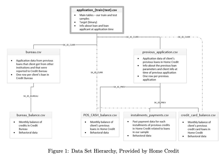
data sets to be analyzed with respect to the, ”application,” data set individually if so desired. These data sets are:
POS CASH balance - “[The] monthly balance snapshots of previous POS (point of sales) and cash loans that the applicant had with Home Credit.”
installments payments - ”[The] repayment history for the previously disbursed credits in Home Credit related to the loans in our sample.”
credit card balance - ”[The] monthly balance snapshots of previous credit cards that the applicant has with Home Credit.”
All three data sets pertain to clients’ ability to spend and save money. In conjunction with the ”previous application,” data set, Home Credit’s goal is to assess their clients’ spending habits, credit usage, and desires to obtain additional lines of credit. For example, these sets could represent a client that has reached their credit limit on previous loans, has withdrawn a sizeable amount of cash from these credit lines, does not make frequent payments on these loans, and is asking for an additional credit limit to obtain more monetary resources. All of these qualities are of import when deciding if a client is going to be approved for another loan, and are thus included in the data analyzed in this project.
Exploratory data analysis (EDA) was performed on the ”application” data set. This was deemed sufficient because it is the parent data set and is considered representative of all data provided.
EDA revealed the presence of outliers, specifically in the time-based features. It also showed that multicollinearity was present among some features. This was observed mostly with the categorical features, and this trend continued throughout the other data sets, as discovered during the feature selection process.
These discoveries prompted the preprocessing of the data in all seven data sets. Firstly, the outliers in the time-based features were dropped, and then the features with missing values were addressed. Removing all features with missing values would drop most features in all data sets, and removing data entries with missing values would severely stunt the amount of data that could be used in this project. However, not removing missing data could affect the accuracy of the model and hinder the understanding of how other features affect the target variable. Therefore, the decision was made to remove some features with missing data, but not all. 50% was chosen arbitrarily as the cutoff for an acceptable amount of missing data in the features. This decision was executed through the removal of all features with 50% or more of their composition containing missing values.
Feature engineering was accomplished with the FeatureTools library. This process was chosen because it eliminated the need to create new features manually with custom classes and functions, and reduced the amount of code necessary to accomplish this task. Deep feature synthesis resulted in the engineering of new features utilizing the following parameters:
Feature Aggregations: Sum, Count, Minimum, Maximum, Mean, Mode
Feature Transformations: Difference, Cumulative Sum, Cumulative Mean, Percentile
After feature engineering, there were 2,370 features in the data set.
electing features that would be utilized by the machine learning models began with once again removing features with 50% or more of their composition containing missing values. This was followed by removing features that contained no non-zero values. There was then an investigation into the extent of multicollinearity among the remaining features. It was found that features with the greatest multicollinearity were mostly categorical. The decision was made to remove features that had a collinearity greater than 0.5.
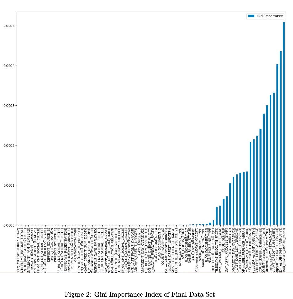
Following feature engineering and collinearity removal, the updated data set comprised 464 features, including original, newly aggregated, and transformed features generated by FeatureTools. For further feature selection, a Random Forest was employed for feature selection, identifying the top 80 features based on the Gini Importance index. This subset of features, chosen for their significance according to the index and its corresponding chart, comprises a mix of both original and transformed features, forming a more streamlined and impactful set for subsequent analysis. The feature families of the final data set are shown in Table 1, and a list of these features is shown in Figure 2.
Next, modeling pipelines were implemented to build robust and effective predictive models on the selected set of 80 most-important features. Two distinct pipelines were constructed to handle numerical and categorical features separately, as shown in Figure 3. The numerical pipeline encom- passed imputation to address missing values and standardization to ensure consistent scales across variables. Concurrently, the categorical pipeline utilized imputation for missing values and one-hot encoding to transform categorical variables into a format suitable for machine learning algorithms.
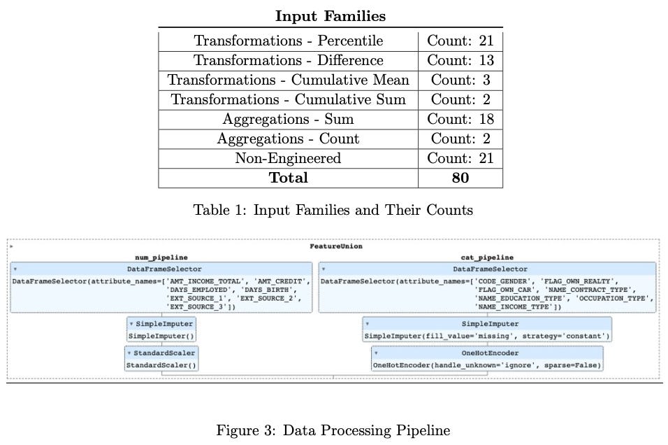
FeatureUnion was then used to integrate the numerical and categorical pipelines. This technique allowed efficient merging of the preprocessed features from both pipelines, ensuring a comprehensive representation of the data set and enhancing the overall predictive performance of the models.
Two models were chosen to analyze and predict data in Home Credit Default Risk. These models were a logistic regression model and a support vector machine model.
The logistic regression model was chosen as the baseline model and included in the experiments because it is capable of accurately predicting classifications and is useful in doing so when the data does not follow a normal distribution. Given the size of the data set, even after feature engineering and selection, a normal distribution could not be guaranteed. The support vector machine (SVM) model was chosen because it also can predict classifications of the data and is still accurate when there is not a normal distribution.
Following the construction of these pipelines, a series of 10 experiments were conducted to optimize hyperparameters for these models. Various combinations of hyperparameters were tested to evaluate their impact on model performance.
The hyperparameters under consideration included those specific to SVM, such as the choice of kernel functions (linear, polynomial, radial basis function, etc.) and the regularization parameter (C), which controls the trade-off between achieving a smooth decision boundary and accurately classifying training data points. For the logistic regression model, hyperparameters like the regularization type (L1 or L2 regularization) and its corresponding strength were explored. Additionally, varying learning rates and iteration limits were considered to optimize the logistic regression models. This meticulous experimentation determined the most effective configuration of hyperparameters for each model.
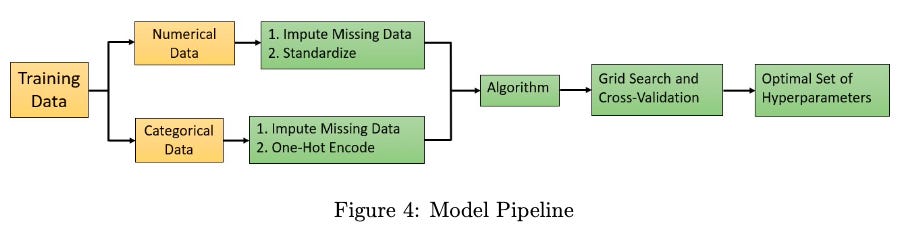
Figure 4 depicts the modeling pipeline utilized to accomplish the tasks necessary.
Part of the evaluation for these models was the use of log loss functions.
For the SVM model, hinge loss, which evaluates the margin between data points and the decision boundary, was used. The hinge loss penalizes misclassifications and aims to maximize the margin while minimizing the classification error. The complete SVM loss function can be expressed as follows:
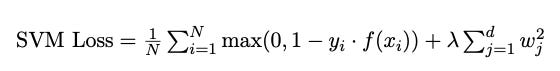
Here, N represents the number of training samples, yi is the true class label for sample i, f(xi) is the decision function output, and λ is the regularization parameter.
For the logistic regression model, the loss function involves the logistic, or sigmoid function to model the probability of a sample belonging to a particular class. The data loss term is typically defined using the cross-entropy or log loss. The complete Logistic Regression loss function can be expressed as:

Here, N denotes the number of training samples, yi is the true class label for sample i, f(xi) is the decision function output, σ is the sigmoid function, and λ is the regularization parameter.
In the modeling efforts, the log loss, also known as cross-entropy loss, serves as a pivotal metric for assessing the performance of both the SVM and logistic regression models. The predict proba method is employed to generate the predicted probabilities for the positive class (class with the label of 1) on the test data set X test. These probabilities are stored in y test prob. Subsequently, the log loss function is applied to assess the consistency between these predicted probabilities and the true class labels (y test).
The neural network utilized similar pipelines, but used ColumnTransformer instead of Feature-Union. This was found to be more appropriate with the requirements of the neural network model.
This model is a Sequential model with two hidden layers, Linear and ReLu, and used Cross Entropy to calculate the loss of the model. A total of 6 experiments were conducted (3 with Adam optimizer, 3 with SGD optimizer) with different epochs and hidden layers.
Results
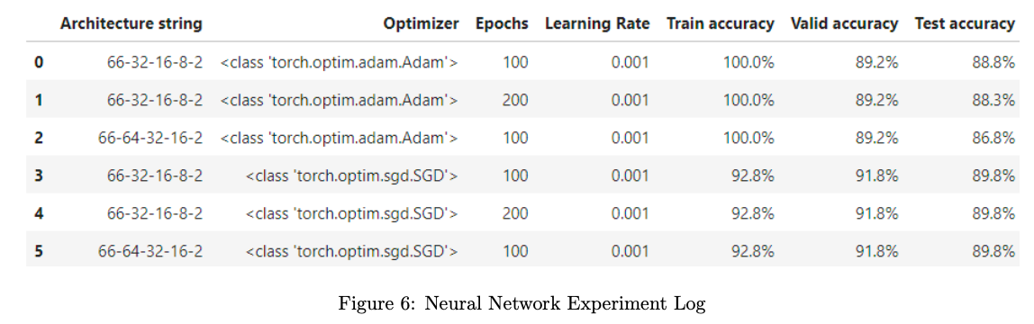
The results of these experiments are visually depicted in Figures 5 and 6, providing insights into the relationships between different hyperparameter settings and their impact on the models’ predictive capabilities.
Discussion
To determine the best model on the selected features after optimizing each model’s parameters, evaluation metrics included Test AUC score, LogLoss and Test Accuracy, in this order, as our criteria for reasons as follows:
AUC is important for the credit risk assessment goal as it provides an indication of how well the models can distinguish between good and bad credit risks. A higher AUC implies better discrimination, which is beneficial for the goal.
LogLoss is important because it penalizes the model for being overly confident and making incorrect predictions. In this case, the models provide probability estimates and therefore LogLoss is an important metric.
Accuracy was examined because it is generally relevant, however the data set is imbalanced. Therefore, additional metrics will be sought in the future.
The outcome of these experiments revealed that the SVM model with a radial basis function (RBF) kernel and a regularization parameter (C) set to 1 emerged as the most effective, demonstrating superior predictive capabilities in assessing credit default risk. This refined pipeline, incorporating the best-performing SVM model, lays a solid foundation for accurate and reliable credit risk predictions in our data science endeavor.
The best neural network model was the 66-32-16-8-2-SGD-100 model with a learning rate of 0.001. It was found that, as shown in the experiment logs, this model produced the same performance as that of the best SVM model. Because this neural network was deployed after the discovery of the SVM model, the SVM model is considered the best model that will be put forth in the Kaggle competition.
The performance of the best model is notably distinct from that of the baseline model, providing valuable insights into the impact of feature engineering and model optimization. The baseline model, a logistic regression classifier applied to the initial set of 205 features before any engineering, exhibited a robust training accuracy of 94.29%, with slightly lower validation accuracy at 88.75%. On the test set, the baseline model achieved an accuracy of 92.65%, a test AUC of 0.72, and a log loss of 0.41.
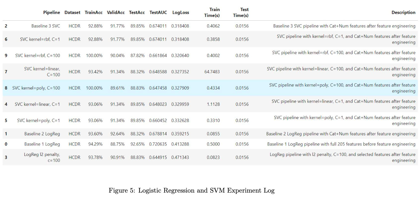
n contrast, the best model, a result of feature engineering and model tuning, demonstrated a lower but still competitive training accuracy of 92.88%, with a higher validation accuracy of 91.77%. However, the test accuracy for the best model slightly decreased to 89.85%, with a test AUC of 0.67 and a lower log loss of 0.31. Despite the trade-offs in accuracy metrics, the best model showcases improved generalization performance and better probability calibration on the test set, suggesting that the feature engineering and model tuning efforts have led to a more refined and effective predictive model.
In the pipelines created for this model, there are several practices done to mitigate the risk of data leakage. In the data preprocessing stage and following feature engineering, the removal of features with missing values exceeding 50% of their composition aided in mitigating this risk. Additionally, during the feature selection process, all missing values were imputed with, ”None,” for ease of use in the data processing pipeline. This pipeline also imputed missing numerical values and one-hot encoded categorical features, further decreasing the risk of data leakage. Finally, extensive multicollinearity analysis ensured independence of the features. Furthermore, the use of a Random Forest with Gini Importance index ensured independence of the features.
Model design also aided in the reduction of data leakage. Provided data was split between training, testing, and validation such that the models were only exposed to the training data set during the learning process. Metrics were therefore calculated for each set separately. Additionally, a random seed was set in the code, allowing for reproducibility. By ensuring the integrity of the data, no cardinal sins of machine learning were committed.
Upon examination of the Kaggle competition scores obtained by other groups within this course, it is evident that the best model presented in this project is also the best model developed in the class. Specifically, the Kaggle public score of 0.5 that was achieved by the best model developed by this project is the smallest score reported by all groups. The next smallest score was 0.73329, meaning that the SVM model discussed here outperformed the next best model by 0.23329. It is suspected that this project’s Kaggle score of 0.5 was achieved through effective feature engineering and selection. Evidence of this is shown in the number of features available for use in the projects and the final number of features utilized. The model presented here appears to have more features available for use, but feature selection was highly successful by providing an appropriate summary of the original data sets without negatively affecting the dimensionality reduction processes.
Conclusion
Through the use of EDA, feature engineering and selection, implementation of machine learning algorithms, hyperparameter tuning, and evaluation, the best model for predicting whether or not clients will repay their loans with Home Credit was developed. The best model, with 80 features after feature engineering and selection, achieved a public and private score of 0.5 in the Kaggle Competition. It was found, through this project, that the best model is an SVM model with an RBF kernel and C=1. The importance of this task was to address the likelihood of repaying loans for clients that previously would not be approved for a loan through Home Credit. It is Home Credit’s desire that these clients be identified such that they can receive loans from Home Credit instead of other, unreputable loaners. With this model, this task has been achieved.